(1724 words)

In this post we will review some of the most basic concepts of Linear Algebra.

Note: the goal of this post is not to teach Linear Algebra from scratch, but rather highlight important concepts in order to help build useful abstractions for more advanced topics or serve as a quick reminder if needed.

Lets get started…

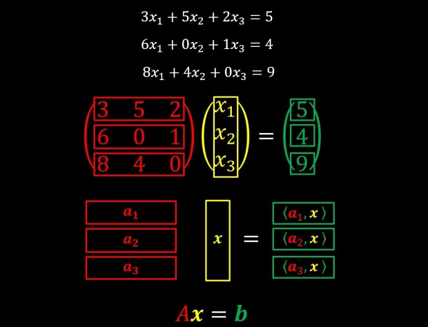
Let us consider the following list of equations below:

They can be re-written as:

As these things turn out a lot here and there, it was useful to define this as matrix multiplication like we can see below:

We can further reduce the notation into:

Where A is a matrix, and x and b are vectors. For our purposes we will consider vectors to be just a list of numbers and matrices to be just a list of vectors (or if you prefer just a list of numbers that are arranged in 2 dimensional grid, what ever works best for you).

Lets now move on to something different, something more geometric in nature, and examine the following plot:

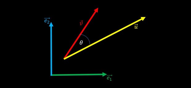
The vectors e₁ and e₂ are the standard Cartesian coordinates and the vectors u and v are just two arbitrary vectors that have angle θ between them.

Lets define the notion of a unit vector:

A unit vector is a vector that is facing to some direction but is of length 1. in this case we mark them with a “hat” instead of an arrow above the letter.

Let’s now define the inner product:

In words, according to that definition, the inner product of two vectors is the product of their magnitudes (or lengths) multiplied also by the cosine of the angle between these two vectors (in this case θ).

Now let’s draw a new purple vector and ask ourselves how can we write it in terms of the existing vectors we already have (e₁,e₂,u,v)?

In words, the purple vector is a projection of the vector v onto the vector u. if you remember your trigonometry classes from high school, you will remember that the magnitude (or length) of the purple vector will therefore be given by the magnitude of the vector v multiplied by the cosine of the angle θ. we can therefore conclude that the purple vector is a vector that is facing the direction of the yellow vector u, and it’s magnitude is given by the magnitude of the red vector v multiplied by cosine of θ.

In math:

If we recall, the cosine of  θ is also given by the inner product between two unit vectors.

As an exercise, let’s now think how we can write also the vectors u and v in terms of the vectors e₁ and e₂?

Recall that u and v are just points in a two dimensional space and if we know, for example, the coordinates of u (lets say u = (u₁,u₂)) then we can think of it’s direction in space as “first go u₁ steps to the right, and then go u₂ steps upwards”. In math, this will correspond to:

With this, we can do the short mathematical derivation of:

The angle between two identical vectors is zero and therefore the cosine of this angle is 1, the angle between two perpendicular vectors is 90 degrees and therefore the cosine of this angle is 0. from this, because e₁ and e₂ are perpendicular and e₁ and e₁ are identical. (as well as e₂ and e₂ which are also identical) one can write:

This is a little reminiscent of how we previously defined matrix multiplication.

So let’s look at this in the following way:

 

It’s now much clearer why I previously mentioned that a matrix is just a list of vectors. To conclude so far, the operation of matrix multiplication is simply serially calculating the inner product between a list of vectors (in the above case, the vectors a₁,a₂,a₃, that together we call them matrix A) and an additional vector (in the above case vector x) and the resulting list of numbers is the output vector (in the above case vector b). Keep in mind that the operation of inner product has also a geometric interpretation, and therefore this list of algebraic equations that we wrote as matrix multiplication has also a geometric interpretation.

To further understand this geometric interpretation, let’s consider the following plot:

In this plot we have 5 vectors. As previously, the vectors e₁ and e₂ are the standard Cartesian coordinates system. The vectors b₁ and b₂ are a rotated version of e₁ and e₂. b₁ is e₁ rotated by 45° leftwards. b₂ is e₂ rotated by 45° leftwards. and v is just an arbitrary vector pointing in the direction (v_1,v₂).

Let’s now look at the projection of v onto the two coordinate systems separately:

Since we can express b₁ and b₂ in units of e₁ and e₂ let’s explicitly write down the inner products between b₁ and b₂ against v.

Interestingly enough, notice that:

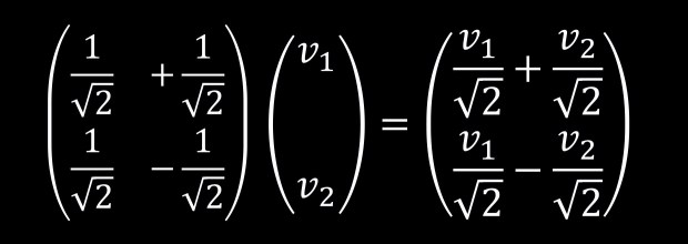
This is of course not a coincidence since:

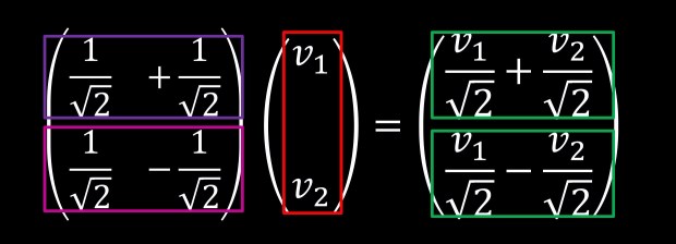
And this we can also write as:

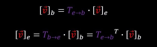
Let us summarize in words: if we want to calculate the projection of the vector v on a new basis, we can do this by multiplying v with a matrix B, whose rows are the new axes of this basis (in this case b₁ and b₂). This means that multiplying a vector by an orthogonal matrix (it’s rows are perpendicular to each other and the length (norm) of each row vector is 1) can be interpreted as representing the same vector in a new basis. Therefore, we can call orthogonal matrices as basis transformation matrices and this is an extremely important concept that is constantly being used throughout the academic literature. If this is not yet the case, it’s well worth putting the time and hammering down this concept until it sits in your head in a completely abstract form:

If we take any vector v that is represented using some basis (in our case {e₁,e₂}) and multiply it by an orthogonal matrix this is equivalent to applying an operation that is representing the same vector v in a new basis (in our case {b₁,b₂}). And the rows of this orthogonal transformation matrix are the new basis elements.

An interesting fact about orthogonal matrices, is that they are easily inverted. in order to invert an orthogonal matrix, you simply transpose it. And equivalently, multiplying a vector by the inverse of a transformation matrix, it is equivalent to applying the inverse transformation. in our case:

For the sake of completeness, let’s complicate life a little bit further and examine the following figure:

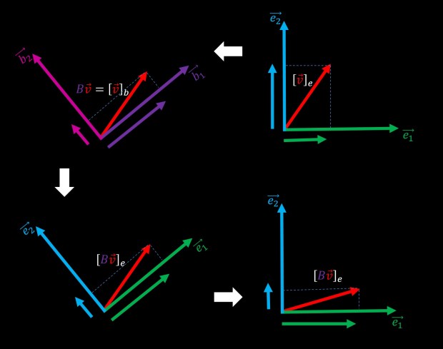
The upper two plots are something we’ve already seen. but consider for a moment the possibility of not thinking about the output of the multiplication of v by B as coordinates in the basis {b₁,b₂}, but rather as coordinates in the original basis {e₁,e₂}. we can see this interpretation on the bottom left plot. The bottom right plot is exactly the same but rotated to be aligned with the top right plot. So, we can see that if we decided to “stay in the same basis”, multiplication of the matrix B has changed the output vector Bv. more precisely, it’s the original vector v after being rotated. This figure tries to illustrate the fact that changing the basis can be seen as rotating the coordinate system and that matrix multiplication can also be seen as rotating vectors in the original coordinate system.

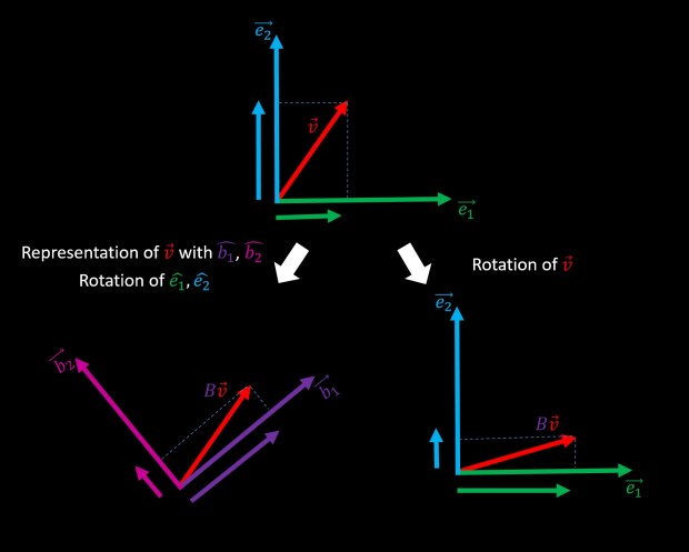
Let’s visually summarize all possible geometrical interpretations of the simple algebraic operation of “multiplying vector v with orthogonal matrix B“:

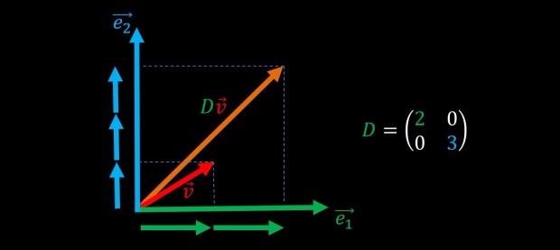
before we move on to discuss eigenvalues and eigenvectors, let’s briefly discuss the simple case of multiplication of a vector by a diagonal matrix:

As we can see, a diagonal matrix D is a matrix whose elements are all zero except the terms on the diagonal, and when it multiplies a vector v, it just scales the elements of that vector by the elements on the diagonal. This operations is often termed “scaling” or “stretching” since it basically just scales or stretches every axis of the original vector:

So thus far we have gathered some intuition of what it means to multiply a vector by an orthogonal matrix and a diagonal matrix. But what about just some arbitrary matrix that is not diagonal nor orthogonal? Well, it turns out that any matrix A that is full rank can be decomposed into a multiplication of diagonal and orthogonal matrices. (a full rank matrix is a matrix whose rows span the entire space, or alternatively non of it’s rows is a linear combination of the other rows, or in other words non of it’s rows are redundant)

Such that U is an orthogonal matrix and Λ is a diagonal matrix.

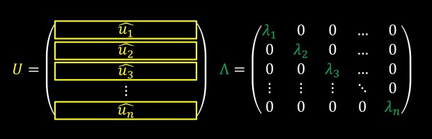
The rows of matrix U, u₁,u₂,u₃,… are usually termed eigenvectors and the diagonal elements of matrix Λ, λ₁,λ₂,λ₃,… are usually termed eigenvalues. We will not go into why they are called this way or how to calculate these values, since any software package will just calculate them for you with a single function call, but we would rather focus on the geometric interpretation of this decomposition.

Recall that multiplying a vector by an orthogonal matrix can be thought as representing it using a new basis

Therefore the following two lines are equivalent

Recall that multiplying a vector by the transpose of an orthogonal matrix is like applying the inverse transformation on that vector

And therefore the following two lines are also equivalent

Which means:

In words, what this means is that the operation of multiplying with matrix A is equivalent to multiplying with matrix Λ but under the representation of basis U.

Put differently, applying the transformation A on vector v is like first projecting v on to basis U, then applying simple diagonal stretching and then projecting back onto the original basis.

This can also be viewed as rotating the vector v, then applying stretching and then rotating back in exactly the opposite direction from the first rotation.

All of these views are completely equivalent, and if they don’t yet sit comfortably in your head, make sure to take the time to go over it again (and again and again) until they do. your future self will thank you as this will come up all over the place.